
Mall Customer - Machine Learning(R)
About This Project
In this task we will analyse and explore the data set “Mall_Customers” which contains basic information about customers at a specific mall. The data consists of five variables; customer id, gender (male or female), age, annual income and spending score, respectively. Since there is no clear indication regarding what the dependent/response variable of the data is, the best way to analyse the data from a machine learning perspective is through unsupervised learning. The goal is first to visually explore the data set and then execute a K-means algorithm to cluster the customer segmentation. This can help provide insights as to what type of customers the mall might want to target in the future. The analysis will focus on the last four variables for our data exploration and the last three for our K-means algorithm.

Gender Comparisons
males: 112
females: 88
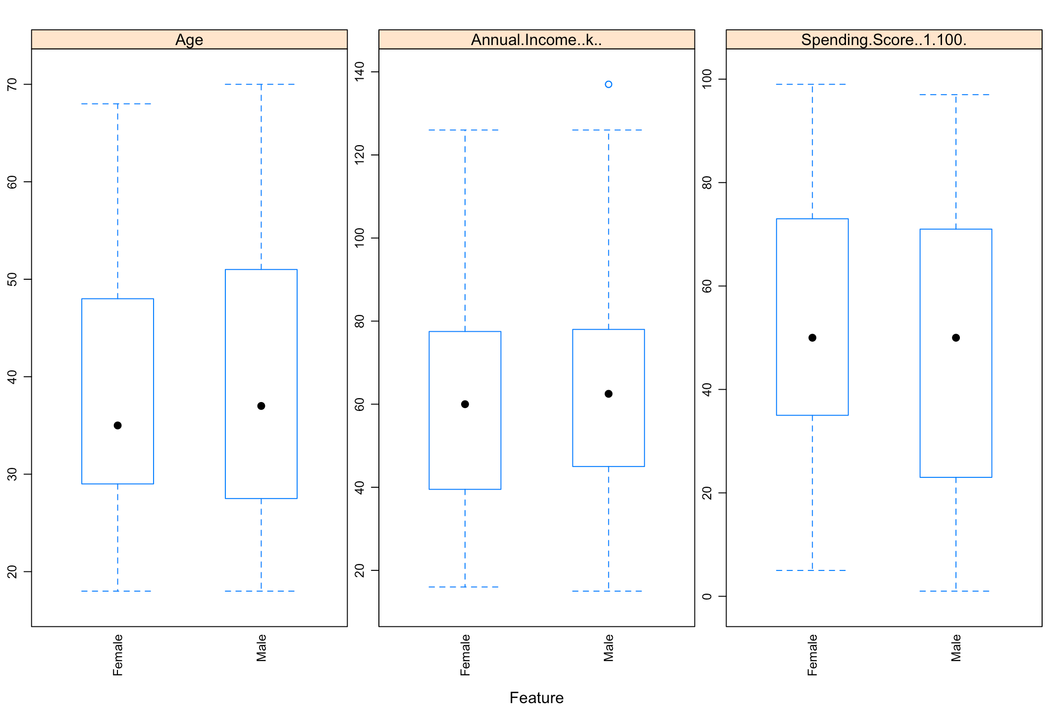
Features Plot
Using the function featurePlot the impact of gender on the variables of age, income and spending score can be visualised as box-plots.

Spending Score
minimum score: 1
maximum score: 99
mean score: 50.2
median score group: 40-50
Mall Customer Segmentation

Age
minimum age: 18
maximum age: 70
average age: 39
median age group: 30-35

Income
lowest income: £15,000
highest income: £137,000
mean income: £65,560
median income: £70,000-80,000
The distribution of income display a relatively normal distribution.
K-Means Algorithm
Before attempting to cluster the data, it is important to try and deduce what the optimal number of clusters should be for our data set. Although there are various methods to determine this, plotting an elbow graph is a method that is widely recognised as suitable. The factoextra and NbClust packages allow for a quick and easy plot of the elbow graph through the fviz_nbclust function, by plotting the number of clusters against the total within the sum of squares.
Deciding the optimal number of clusters from the elbow graph depends on where the “bend” of the graph is. If there is not a distinct bend in the graph, like for the one above, the optimal number of clusters is decided to the k in which the total within the sum of squares is not reduced by much more going to another k. For our plot, that number is k = 6.

Unsupervised Clustering
After deciding on the optimal number of clusters, the kmeans function from the stats package is applied to the three numerical variables; age, income and spending score respectively, and the ggplot function is used to plot our clustering results.The ggplot allows for visualization of the different clusters.

Observations:
Cluster 1 are customers who have a relatively large income, but low spending score.
Clusters 2 and 5 are customers who have a medium-income and medium spending score.
Cluster 3 represents customers with low income and a low spending score.
Cluster 4 represents customers with a low income and high spending score
Cluster 6 represents customers with a high income and a high spending score.
The mall wants to make sure they address the needs of the customers belonging to both of these clusters to make sure they can retain them. The visual cluster analysis of age vs. spending score does not provide much value to the mall, however methods such as age-specific functionality/service upgrades could perhaps increase the spending score of certain customers.

Observations:
The visual cluster analysis of age vs. spending score does not provide much value to the mall, however methods such as age-specific functionality/service upgrades could perhaps increase the spending score of certain customers.
Conclusion
Through the data exploration and k-means algorithm completed above, it is clear that there are no real outliers or surprising findings. Age, income and spending score are distributed as expected, and the effect of gender on these does not cause much variation. The K-means algorithm produces six customer clusters which the mall management may find useful for future expansion and marketing targeting.